Measurement of the chemical composition of ancient coins with portable XRF
Abstract:
The elemental composition of antique coins is
of great interest in the field of numismatics. An obvious quick
and easy method to investigate these artifacts is X-Ray
fluorescence, especially using portable spectrometers, although
these spectrometers are limited in terms of precision and
accuracy of the measurement results. In this work some
shortcomings of XRF‑spectrometry were investigated. A crucial
point is that enough single measurements should be taken to
obtain meaningful averaged elemental compositions, leading to an
increase in precision. Further, correction factors were derived
to improve accuracy, so that overall, the set of data will be
improved regarding both precision and accuracy. These correction
factors were based either on reference samples or on
simulations, thus demonstrating the feasibility of deriving
meaningful correction parameters for defined sets of coins.
Although portable XRF can possibly not replace
high-precision/high accuracy measurements like ICP-MS, we show
that nevertheless results, especially when obtained from a set
of samples and from multiple measurements of one and the same
sample, can be used to differentiate the material nature of
uniform groups of coins, e.g. to find correlations between trace
element concentrations or to identify clusters. Thus, portable
XRF provides easy access to measurement of high sample numbers
with the potential to discover yet unknown trends in
composition, e.g. in numismatic collections.
Keywords:
X-ray fluorescence spectrometry (XRF), XRF
correction factors, XRF simulations, surface roughness, Roman
billon coins, lead-bronze coins
Zusammenfassung:
Die elementare Zusammensetzung
antiker Münzen ist in der Numismatik von großem Interesse.
Eine einfache und schnelle Methode ist die
Röntgenfluoreszenzspektrometrie, besonders mit portablen
Geräten, wobei die Genauigkeit und Richtigkeit der Resultate
limitiert sind. Einige dieser Limitierungen wurden in dieser
Arbeit genauer untersucht. Um aussagekräftige gemittelte
Elementkonzentrationen zu bestimmen, sollte die Zahl der
Einzelmessungen groß gewählt werden. Eine höhere Genauigkeit der
Daten lässt sich generell durch eine höhere Anzahl an
Einzelmessungen erreichen. Durch Korrekturfaktoren lässt sich
auch die Richtigkeit verbessern; diese wurden in dieser Arbeit
über zwei verschiedene Herangehensweisen ermittelt. Zunächst
wurde ein Korrekturfaktor über Referenzproben mit bekannter
Elementkonzentration ermittelt. Anschließend wurde ein weiterer
Korrekturfaktor über ein Simulationsprogramm bestimmt. Die
Röntgenfluoreszenzspektrometrie kann mithilfe dieser
Korrekturfaktoren insgesamt richtigere und präzisere Messwerte
liefern, wird jedoch hochpräzise und richtige Methoden, wie
ICP-MS, nicht ersetzen können. Die Möglichkeit, viele
Einzelmessungen in kurzer Zeit durchzuführen, erhöht aber die
Präzision und die Korrekturfaktoren erhöhen die Richtigkeit der
Datensätze. Insgesamt ist dies hinreichend für eine Untersuchung
von einheitlichen Münzgruppen, z. B. im Hinblick Korrelationen
von Spurenelementen mit Hauptkomponenten. Damit bietet die
portable Röntgenspektrometrie einen einfachen Zugang zur Messung
großer Münzgruppen und die Möglichkeit, bisher unbekannte Trends
in Zusammensetzungen zu finden.
1. Introduction
1.1. Methods for elemental analysis of
historical artifacts
In archaeology many
different characteristics of an artifact are of interest. One of
these characteristics is the elemental composition of
artifacts, which is the concentration of the chemical elements
within the artifact. Knowledge of element composition can help
assign the sample to a specific era or provide information about
the provenience, production methods, or raw materials use[1].
In general, such an elemental analysis might be performed with
destructive, semi‑destructive and non‑destructive methods. Using
destructive analytical methods, a sample is consumed during the
measurement process. However, the size of the sample may be very
small, so that only minor damage needs to be inflicted on the
artifact. Central concepts for the comparison of different
analytical methods are accuracy and precision of measurements
are of great interest (see figure 1).
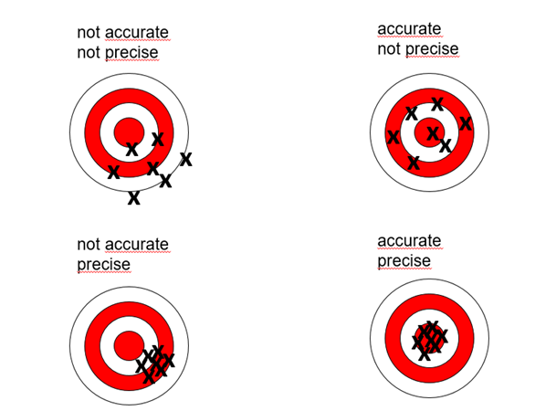
Some analytical methods
deliver both precise and accurate data, some are only yielding
either precise or accurate data, and some methods are limited in
both precision and accuracy. Destructive methods like
inductively coupled plasma mass spectrometry (ICP-MS)[2]
or inductively coupled plasma optical emission spectroscopy
(ICP‑OES)[3]
can very precisely determine the elemental composition of the
sample, based on sample sizes in mg or even in the sub-mg range[4].
With a suitable calibration, these measurements will also
provide high accuracy. With a laser coupled to the spectrometer,
laser-ablation inductively coupled plasma mass spectrometry
(LA-ICP-MS)[5],
samples can e.g. be taken from a small spot of a historical
artifact with a diameter of less than 0.1 mm and only a few µm
deep. In this sense, LA‑ICP‑MS might be called
›semi‑destructive‹ as such a spot is barely visible to the naked
eye on a bigger artifact. Nevertheless, the artifact is not
unharmed in a strict sense, so curators might remain skeptical
of such a method. LA-ICP-MS needs no chemical sample treatment
and therefore consecutive measurements can be made in short
time, but its use remains limited due to the fact than an
LA-ICP-MS is not a portable instrument. Artifacts that are to be
measured must be brought in a scientific lab and despite its
virtual non‑destructiveness, decisions of collection curators
are needed to prevent or mitigate unnecessary influence on the
artifacts. Although environments do exist, that foster such
close relationships between humanities and scientists as the
CRNS lab collaborating with the Louvre museum[6],
this is rather an exemption. On the other hand, there is a broad
range of spectroscopic techniques that are in general
non-destructive, e.g. nuclear magnetic resonance (NMR)[7],
infrared spectroscopy (IR)[8],
as well as X-ray fluorescence (XRF)[9],
that are all radiation based and have been successfully applied
to historical artifacts. All these methods can be highly precise
and have the potential for high accuracy, if calibrated. Also,
Neutron activation analysis (NAA)[10]
can be classified as a non‑destructive method. Although NAA
might lead to an activation of the sample during the
investigation (i.e. the generation of a small amount of
temporary or permanent radioactivity), the method has been used
successfully multiple times[11].
One advantage of NAA is that it can be calibrated relatively
easily because matrix effects in the calibration are mostly
negligible. Of the different spectroscopic methods, XRF is to be
highlighted: XRF can deliver the elemental composition of a
sample in a non-destructive way, there is a broad experience
analysis of artifacts with different X-ray sources[12]
and second, small portable XRF spectrometers that can be used
within the museum context are available for several years[13].
In these devices, a small X-ray tube is used to irradiate the
sample, and the equipment is small and light enough to place it
on a simple tripod in any orientation. Hence it can be applied
as well as to artifacts of any size or paintings without even
moving them out of an exhibition environment. However,
especially portable XRF is limited in both accuracy and
precision, because both might be influenced by the sample
geometry (e.g. surface structure and roughness). Generally,
X‑ray fluorescence might also be induced using a particle beam
(PIXE, for particle induced X‑ray‑emission)[14]
or the strong radiation of a synchrotron source[15]:
Both methods can be advantageous under different circumstances
but are not portable.
However, the limitations
of XRF that might hamper widespread use are:
- XRF
works better with heavier chemical elements, i.e. it is not
well-suited for the analysis of the main components of
organic materials,
- possible matrix effects
influence the accuracy of the results, i.e. the accuracy
might decrease, especially if the object contains multiple
chemical elements,
- measurement results,
especially precision, might be influenced by the sample
surface geometry, as will be explained in more detail below,
- XRF is generally not a
high accuracy method, also depending on the sample
composition,
- measuring depth and width
are limited, giving inconclusive results in the case of
inhomogeneous materials.
With this work we want
to show that XRF can be successfully applied when:
-
light chemical elements play no role (like in metal alloys),
- matrix
effects can be minimized using suitable calibration methods,
- the
influence of sample geometry can be estimated by a model,
- high
accuracy is not decisive e.g. for analyzing groups of
artifacts, i.e. when several subsets of samples are compared
to each other,
- when
enough measurement points are used, yielding a
representative (and thus more precise) composition for a
single object and allowing for a statistical approach when
several samples are measured.
We will demonstrate this
throughout this paper on the example of ancient Alexandrian
coins from the Roman period, lead-bronze coins (drachms) and
billon coins (tetradrachms) of Claudius (41–54 AD) and Nero
(54–68 AD). We will explicitly show how some of the limitations
of XRF can be overcome when measurements on a larger group of
coins (n = 20) are performed and analyzed, revealing new
information. We will show that accuracy as well as precision can
be improved by making use of correction factors and a large
number of single measurements for each coin. While this does not
overcome completely the limitations of portable XRF, with these
procedures data gained from large sample sets (e.g. of coins)
might discover yet unknown trends and provide new insights.
1.2. Aim of this work
In this work, we
describe how the influence of self-absorption on XRF-spectra can
be corrected by introducing a correction factor (improving
mostly accuracy) and how the influence of patina and surface
effects can be minimized with multiple measurements (improving
precision). Self-absorption correction factors were obtained in
two different ways: for lead-bronze coins, we produced and
measured artificial reference samples; for billon coins we
simulated different coins with the program XMI-MSIM[16].
The correction factors obtained were applied to the measured
data of the coins. XMI-MSIM was also used to estimate
measurement uncertainties resulting from geometrical effects
(like embossment).
By these simulations it
is underpinned that the uncertainties resulting from patina or
surface effects are consistent with the statistical uncertainty
obtained from multiple measurements. In contrast to the use of
references samples, simulations with XMI-MSIM are more
versatile. Finally, some actual results from the measurement of
the different coins are discussed.
1.3. Principles,
Possibilities and Limitations of X-Ray Fluorescence spectrometry
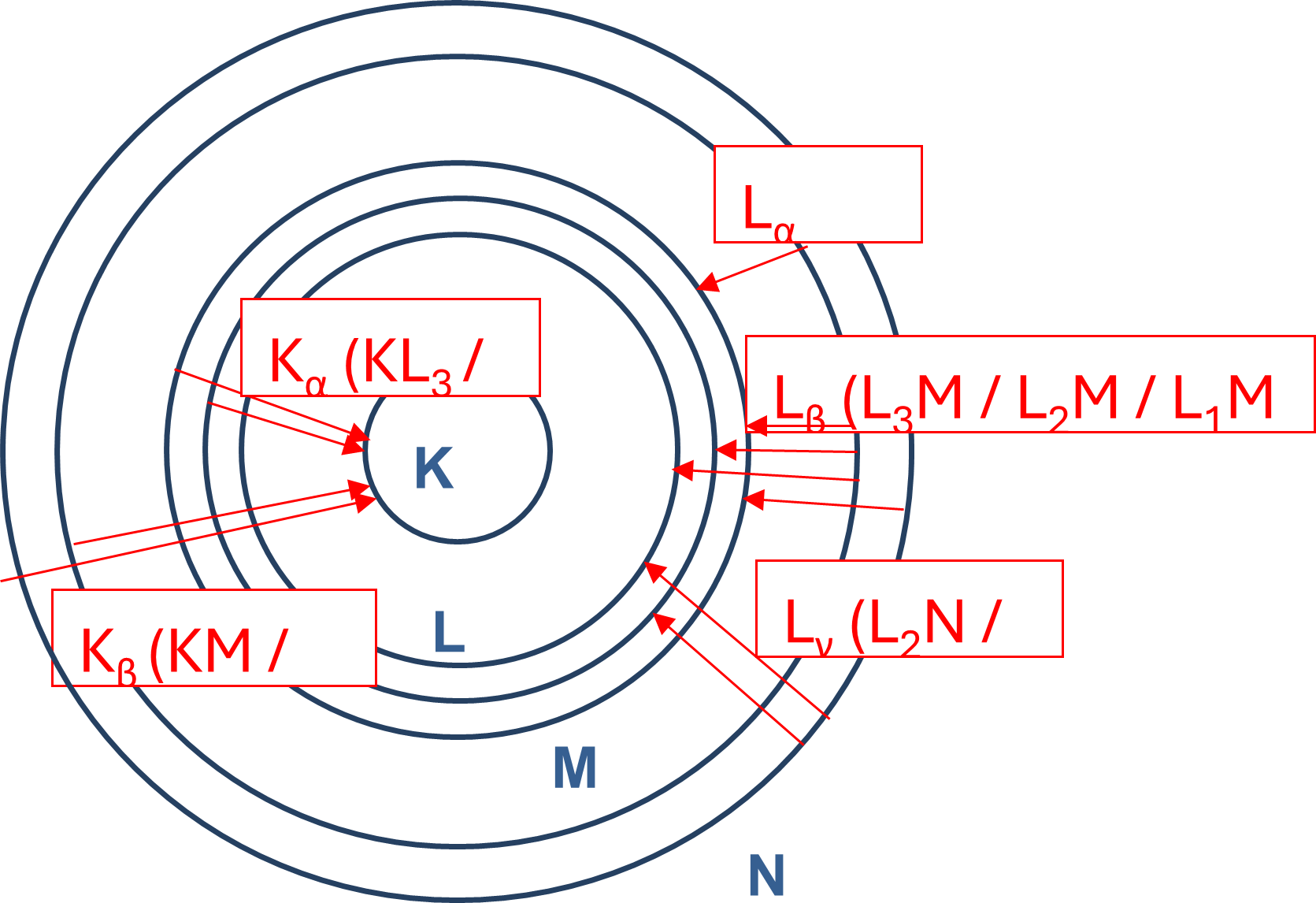
With X-rays, electrons
can be ejected from an atom. This leads to an atom with empty
electronic states. The remaining shell electrons cascade
downwards to reach the empty states. During this process,
characteristic X-ray fluorescence radiation is emitted. This
cascade can be seen in figure 2. Because the electric
field of every chemical element is different, the X-ray
fluorescence radiation exhibits energies that are characteristic
for each chemical element, making it identifiable and
quantifiable[17].
The intensities of these characteristic X-rays can be used to
calculate the elemental composition of the sample under
consideration[18].
However, for an accurate quantitative measurement both the
attenuation of the incoming and outgoing radiation within the
sample itself must be considered. Especially, fluorescence
(outgoing) radiation might be absorbed again by another atom and
thus cause secondary fluorescence, while at the same time the
intensity of the primary radiation decreases. This results in a
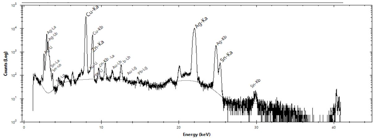
loss of accuracy for the measurement. Figure 3 depicts a
typical X-ray fluorescence spectrum obtained from a coin of the
Claudius era. The coins of the Claudius and Nero era that were
investigated are billon coins, an alloy containing the main
elements Cu and Ag. Visible in the spectrum are the K-Lines of
Cu and Ag which are the most dominant. Furthermore K- and
L-lines of other elements e.g. Au, Sn, Zn and Fe are also
visible.
In general,
XRF-spectrometry is an easy and fast method to investigate
samples. A measurement time of only a few minutes already
delivers meaningful results. This allows for a larger number of
samples to be investigated with multiple measurements on each
object thereby yielding a large set of statistical information.
This means an increase in data precision. The obtained data
enables, for instance, the classification of samples into
distinct groups as well as the recognition of overarching trends
among them.
1.4. Measurement of
coins with portable XRF
Coins are generally
suitable objects for XRF because they are made of characteristic
metals or alloys. Elements with an atomic number lower than 11
(sodium, Na), which cannot easily be detected by XRF, are
generally no main elements in coins. Although coins are a good
example for a sample group containing many similar objects that
can be compared on a statistical basis, XRF-measurements are
done more commonly on paintings or papyrus inks. In those cases
the analysis is simpler and therefore more accurate, because the
above-mentioned self‑attenuation in the sample can be neglected.
This is due to the limited thickness of the paint in those
objects. In contrast, the measurement of coins might not only be
influenced by self-attenuation, but also by the presence of
patina, or geometric effects (surface roughness) that must be
considered. The penetration range of X-Rays may vary, depending
on the X-Ray-source used but usually represents a penetration
depth of 0.1 mm up to 1 mm. Therefore XRF-measurement data may
not represent the core of a coin, but certainly the penetration
depth of the X-Rays will be portrayed accordingly. The core of a
coin may differ in its composition form the outer composite
layers, but according to Ernst Gölitzer[19]
a correlation between core material and outer layers seems
plausible and would make vague assumptions about the overall
material possible.
Patina effects on the
measurement
Often coins build up a
patina. Most materials are not resistant to oxidation or
corrosion, thus forming a thin chemically modified surface
layer. This patina might in general influence an XRF-measurement
as the penetration depth of X‑rays is typically on the scale of
several µm (depending on the element mixture of the sample and
the exact energy of the X‑rays). In principle, it is possible to
correct measurements for patina effects[20].
But because the patina is mostly made up of oxides and therefore
the density of that material is typically lower compared to the
bulk material, the absorption of X-rays is lower in the patina
than the rest of the coin. Especially when several objects can
be compared on a statistical basis, patina effects play only a
secondary role. Hence, exact determination of the elemental
composition is challenging. A removal of the patina must be
considered destructive and should therefore be avoided. However,
as we will show below, in practical cases the patina might
increase measurement uncertainty, but if several measurements
are performed on the same object, these uncertainties can be
quantified, and a comparison of objects is still possible. This
means that the uncertainties resulting from a patina may be
somewhat fixed in a statistical way by a large set of data,
while a single data point will still be lacking in precision.
Self-absorption and
secondary fluorescence
There are several
influences on XRF-measurements. The size (solid angle) and the
efficiency of the detector have an influence on the measurement,
as well as the attenuation of the incident beam, the probability
of photon creation, and the attenuation of the induced
fluorescence radiation. As described above, additional X‑ray
fluorescence can be induced via secondary absorption inside the
sample itself. The characteristic fluorescence of a heavy
element can induce characteristic fluorescence of lighter
elements in the sample, leading to an overrepresentation in
intensity of the lighter elements compared to the heavier
elements. Accuracy is negatively affected by secondary
fluorescence. All these effects might be corrected collectively,
in our works using either reference samples or computational
simulation of XRF‑measurements.
Surface
irregularities
In addition to patina
effects and self-absorption as well as secondary fluorescence,
the geometric structure of the sample may influence the result
of an analysis. The point is that the attenuation of the X-rays
depends on the surface geometry (e.g. the embossment of the
coins) of the samples. If the surface of the sample is
structured, X-rays must travel through more or less coin
material, depending on the incoming angle and outgoing angle of
radiation (see figure 4).
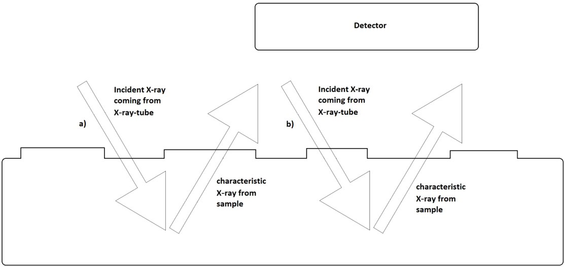
Because different
elements have different absorption coefficients and the
penetration depth is also dependent on the energy the elemental
X-rays have, the intensity of the X‑ray can differ and lead to
an additional uncertainty of the elemental composition. Although
this behavior is difficult to treat in a mathematically exact
way, we will show that the influence of this effect on the
result can be estimated and can be partially overruled by
performing several measurements on each sample, improving
precision.
2. Experimental and
Results
2.1. Coins under
investigation
In this work, a total of
43 coins were measured with a portable ELIO SN 1254
XRF‑spectrometer, 20 random lead-bronze coins from the Roman
period and 23 billon coins (tetradrachms) issued under Claudius
and Nero, respectively. Also, we chose silver coins
for the second part of the paper, because silver coins from the
early years of Claudius and Nero, between the reintroduction of
silver coinage by Tiberius and the Neronian reform, have been
underrepresented in literature so far. The main components of
the lead-bronze coins are Cu, Sn and Pb; the main components of
the billon coins are Cu and Ag. All coins stem from the coin
collection of the Department of Classics of the University of
Cologne and are listed in table 1 according to their
inventory numbers.
|
Lead-bronze coins |
Billon coins Claudius |
Billon coins |
|
AL_0039 |
ALSK_0047 |
AL_0187 |
|
AL_0093 |
ALSK_0048 |
AL_0188 |
|
AL_0417 |
ALSK_0058 |
AL_0189 |
|
AL_0537 |
ALSK_0059 |
ALSK_0169 |
|
AL_0563 |
ALSK_0060 |
ALSK_0170 |
|
AL_0609 |
AL_0061 |
ALSK_0171 |
|
AL_0654 |
AL_0062 |
|
|
AL_0701 |
AL_0063 |
|
|
AL_0815 |
AL_0064 |
|
|
AL_0954 |
AL_0065 |
|
|
AL_1179 |
AL_0075 |
|
|
AL_1305 |
AL_0076 |
|
|
AL_1359 |
AL_0081 |
|
|
AL_1491 |
AL_0082 |
|
|
AL_2210 |
AL_0086 |
|
|
AL_2291 |
AL_0087 |
|
|
AL_3375 |
AL_0088 |
|
|
AL_3386 |
|
|
|
AL_3404 |
|
|
|
AL_3468 |
|
|
2.2. Artificial
reference samples
To derive correction
factors for lead-bronze coins experimentally (see section 3.1.1
below), we produced 42 samples with known ratios (wt%) of Cu, Sn
and Pb (see table 2). The ratios of the metals were
selected such that they cover typical compositions of
lead-bronze coins.
|
Cu amount /
wt% |
Sn/Pb amount
/ wt% |
||||||
|
70 |
0/30 |
6/24 |
12/18 |
15/15 |
18/12 |
24/6 |
30/0 |
|
75 |
0/25 |
5/20 |
10/15 |
12.5/12.5 |
15/10 |
20/5 |
25/0 |
|
80 |
0/20 |
4/16 |
8/12 |
10/10 |
12/8 |
16/4 |
20/0 |
|
85 |
0/15 |
3/12 |
6/9 |
7.5/7.5 |
9/6 |
12/3 |
15/0 |
|
90 |
0/10 |
2/8 |
4/6 |
5/5 |
6/4 |
8/2 |
10/0 |
|
95 |
0/5 |
1/4 |
2/3 |
2.5/2.5 |
3/2 |
4/1 |
5/0 |
|
|
Copper (Cu) |
Tin
(Sn) |
Lead (Pb) |
|
Producer |
Alfa Aesar |
Acros Organics |
Alfa Aesar |
|
|
|
|
|
|
Purity |
99% |
99.5% |
99.95% |
|
Grain size |
~100 Mesh |
~100 Mesh |
~100 Mesh |
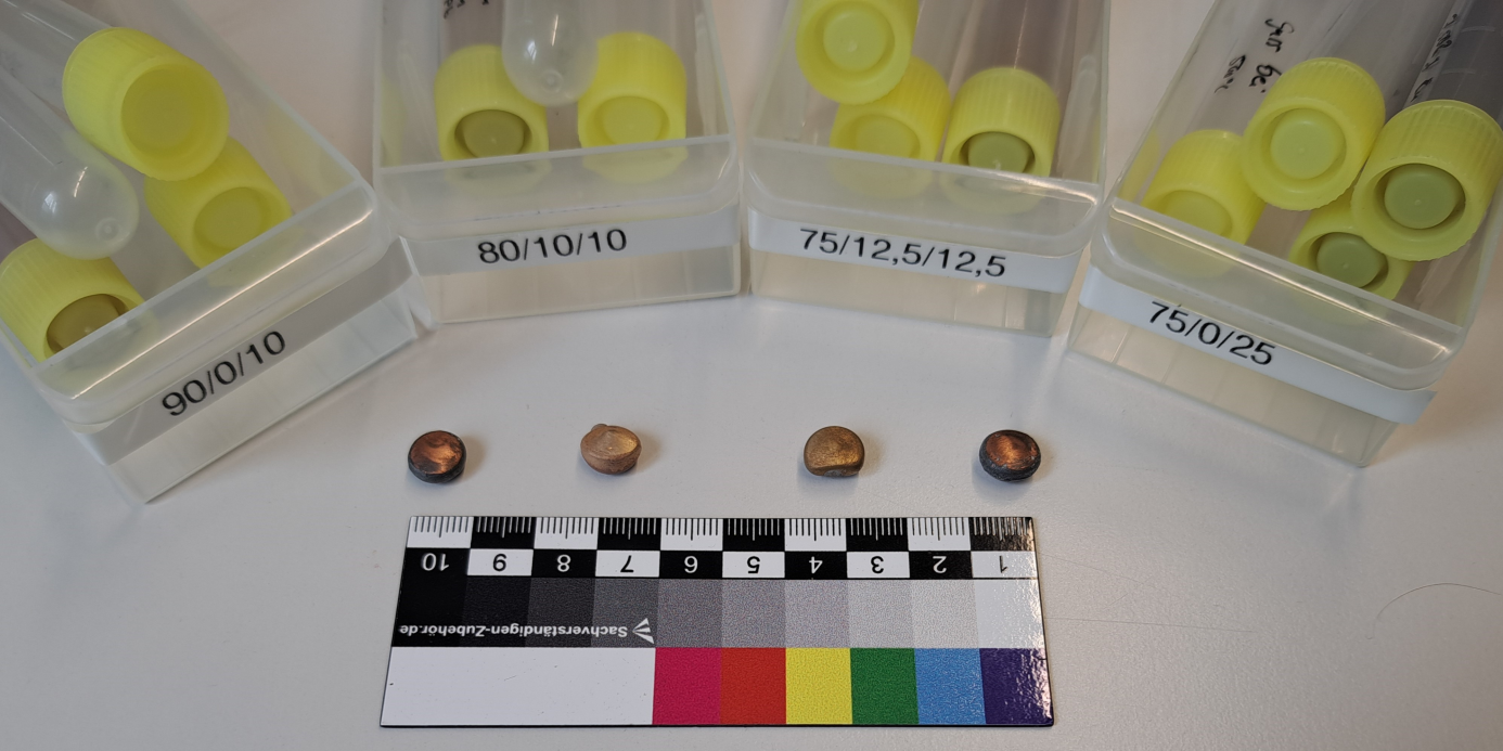
The amount of Cu varied from 70 to 95 wt%, reflecting the range of historical lead-bronze. The remaining wt% of the sample is split between Sn and Pb also in varying amounts. The powdered pure metals were weighed, mixed in their powdered form and melted for 3 hours without mechanical mixing at 1050 °C in graphite crucibles. This was done to ensure a homogenous melt to produce a coin-like form. It was verified by weighing that material loss due to evaporation was negligible. All in all, 42 different samples were produced. Figure 5 below shows 4 of these reference samples.
2.3. XRF measurements
To obtain a set of data
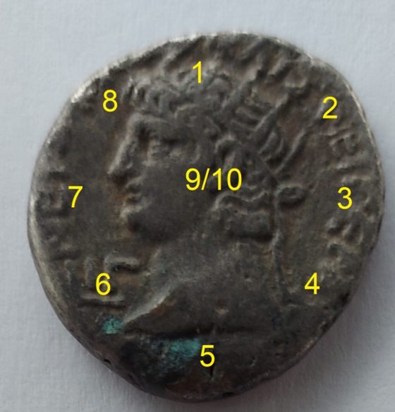
for each coin that was measured, ten different measurements were
done on each coin side. 8 measurements were taken along the rim
of the coins and 2 measurements in the center. Measuring spots
can be seen in figure 6.
The measurements of
coins and reference samples were done with the ELIO device, and
the composite analysis was done by the ELIO software. To obtain
a more precise data set, only the expected or probable elements
of these coins were investigated (i.e., selected as possible
components in the analysis software). These were Cu, Ag, Pb and
Sn as main components as well as Zn, Fe and Au as secondary
components. The reference samples were measured in the same
manner as the billon and lead-bronze coins.
3. Results and
Discussion
3.1. Correcting
measurement data based on reference samples
As described above, to
correct the X-ray intensities of the different elements for
self-attenuation and secondary fluorescence in coins (or general
in thicker samples), correction factors are needed. Such factors
can either be developed experimentally or from simulations. In
this work both methods were used as described in the next
paragraphs.
3.1.1. Correction
factors (experimental)
A correction factor for
the measurement of Pb/Cu in lead-bronzes was derived
experimentally. This was done to enhance accuracy of XRF. The 42
reference samples (section 2.2.) were measured with XRF to
deduce the impact of the different metals to each other. The
measured mass fractions of Cu, Sn, and Pb of all 42 samples were
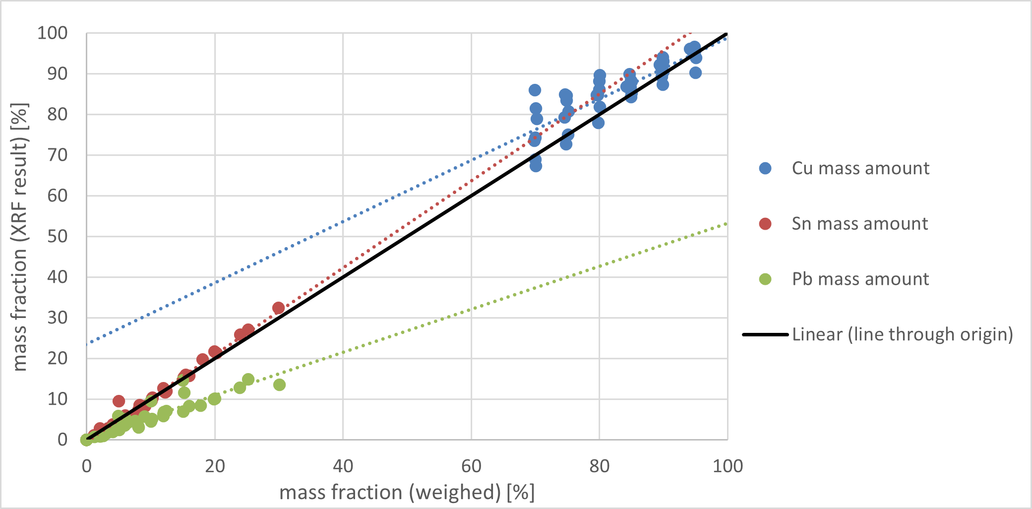
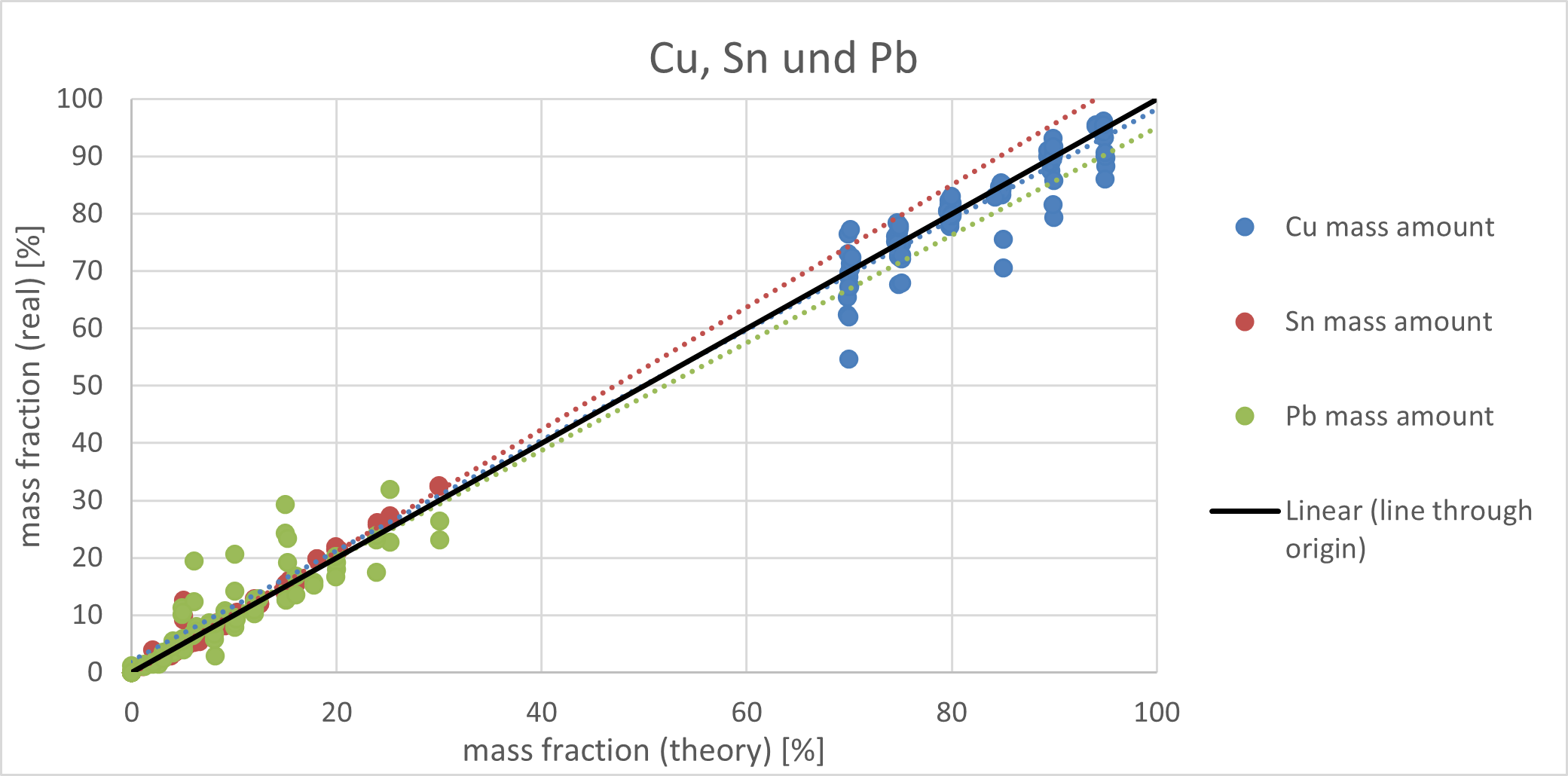
plotted vs. the actual mass fractions (see figure 7). The
measured fractions were taken from output of the ELIO software,
averaged over 20 measurements as described above, to increase
the precision of the data. The actual mass fractions were
calculated from the weightings of the raw materials, see section
2.2. The dashed lines represent linear fits. While the tin mass
fractions are very near to their nominal values, the lead and
copper values deviate. The Pb concentration is obviously
underestimated, and the Cu concentration is overestimated. This
agrees with the assumption that secondary absorption plays an
important role, because the fluorescence radiation of heavier
elements might be absorbed again by lighter elements. Also, the
deviation is linear within the given concentration range.
Therefore, a correction
factor
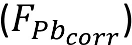 for the wt% value of lead can be
calculated as the reciprocal slope of the linear fit shown in
figure 6. This yields the following correction factor.
for the wt% value of lead can be
calculated as the reciprocal slope of the linear fit shown in
figure 6. This yields the following correction factor.
(1)
= 1.84 ± 0.43
To apply the correction,
the nominal lead content (in %, ELIO software output) is
multiplied by the correction factor. The resulting nominal
elemental concentrations are then renormalized to 100%. If the
resulting values for Cu, Sn, and Pb are plotted again (figure
8), it turns out that not only the Sn data are now fitting
satisfyingly, but also the Cu data. All values are now close to
the bisecting line. No second correction factor is needed in
this ternary alloy. Obviously, lead is underestimated by the
same factor as copper is overestimated. This agrees well with
the assumption that the measurements are mainly affected by
re-absorption of lead fluorescence radiation by copper and the
subsequent secondary copper X-ray fluorescence. From our
experience this correction factor is reliable within the range
of sample compositions under investigation, which is all samples
not containing more than 30 wt% lead, covering the typical
compositions of lead-bronze coins.
3.2. Correction
factor based on simulations
To obtain correction
factors using a simulation, the experimental setup was modeled
within the XMI-MSIM software. All parameters of the experiment
were simulated, such as the properties of the X‑ray‑source,
geometrical conditions, material and geometry of the sample, as
well as material, size and form of the detector. For the
simulations in this work, the X‑ray source and detector were
modeled as given in detail in the supplementary information. As
samples, different billon coins were simulated with varying
Cu/Ag ratios. As during XRF of coins, the X-ray beam is
completely attenuated within the sample, the coins were modeled
as infinitely thick layers within XMI-MSIM. The simulated sample
furthermore contained 1.86 wt% trace elements like Pb, Zn, Sn,
Au and Fe besides the two main elements Cu and Ag, which is a
typical amount of trace elements for billon coins. The
measurement geometry in the first simulation step was modeled
after the geometry of the ELIO device. The resulting spectra
were evaluated within XMI-MSIM, and a correction factor
correcting the ratio of Ag and Cu was to be deduced by comparing
via the simulated X-ray line intensities (details see below).
The amount of trace elements was the same at each simulation
run, while only the ratio of Cu and Ag changed. This specific
alloy composition was chosen to resemble the bulk of the
tetradrachm coins measured via XRF.
The ratio of Cu and Ag
varied from 95/5 to 5/95 in steps of 5 wt% for each element as
can be seen in table 4. In figure 9, the
intensities (peak areas) from the simulations are plotted vs.
the nominal Cu content.
|
1 |
2 |
3 |
4 |
5 |
6 |
|
Cu / wt% |
Ag / wt% |
I(Cu) a.u. |
I(Cu)/(I(Cu)5%) |
I(Ag) a.u. |
I(Ag)/(I(Ag)5%) |
|
93.2 |
4.91 |
95134.3 |
1.69 |
3275.05 |
1.00 |
|
88.3 |
9.81 |
86182.3 |
1.61 |
6438.89 |
0.98 |
|
83.4 |
14.7 |
77981.4 |
1.54 |
9503.02 |
0.97 |
|
78.5 |
19.6 |
70728.2 |
1.49 |
12511.2 |
0.96 |
|
73.6 |
24.5 |
63926.3 |
1.43 |
15420.5 |
0.94 |
|
68.7 |
29.4 |
57644.4 |
1.39 |
18281.8 |
0.93 |
|
63.8 |
34.3 |
51849.7 |
1.34 |
21053.8 |
0.92 |
|
58.9 |
39.3 |
46384.8 |
1.30 |
23784.8 |
0.91 |
|
54.0 |
44.2 |
41322.9 |
1.26 |
26452.9 |
0.90 |
|
49.1 |
49.1 |
36512.7 |
1.23 |
29051.3 |
0.89 |
|
44.2 |
54.0 |
32033.5 |
1.20 |
31664.6 |
0.88 |
|
39.3 |
58.9 |
27709.6 |
1.17 |
34129.9 |
0.87 |
|
34.3 |
63.8 |
23676.2 |
1.14 |
36558.7 |
0.86 |
|
29.4 |
68.7 |
19837.3 |
1.11 |
38982.5 |
0.85 |
|
24.5 |
73.6 |
16135.8 |
1.09 |
41417.9 |
0.84 |
|
19.6 |
78.5 |
12621.9 |
1.06 |
43758.7 |
0.84 |
|
14.7 |
83.4 |
9284.38 |
1.04 |
46004.1 |
0.83 |
|
9.81 |
88.3 |
6066.77 |
1.02 |
48297.8 |
0.82 |
|
4.91 |
93.2 |
2971.09 |
1.00 |
50506.6 |
0.81 |
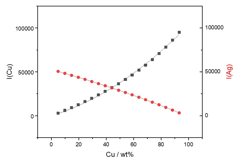
It is clearly visible that the intensities of Cu rise disproportionately with rising Cu content in the sample. The intensity of Ag radiation drops almost proportionately with rising Ag contents. Reason for this difference is probably the contribution of secondary X-ray fluorescence of Cu induced by the fluorescence radiation of Ag, reducing measurement accuracy. To correct this, a correction factor was derived from this data and can be seen in equations (2) and (3).
(2)

(3)
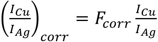
At first all intensities
were normalized to the intensity value of 5 wt% Cu or 5 wt% Ag
respectively. By this, an influence factor can be obtained,
which increases in the case of Cu with rising Cu wt% and
decreases for Ag with rising Ag wt%. By multiplying the
respective intensities with the reciprocal influence factor
corrected Intensities were obtained. Then these corrected
intensities were used to calculate corrected intensity ratios.
The corrected values are given in table 5.
|
Cu / wt% |
I(Cu) |
Ag / wt% |
I(Ag) |
[I(Cu) / I(Ag)]korr |
|
93.2 |
56451 |
4.91 |
3275 |
17.2 |
|
88.3 |
53480 |
9.81 |
6550 |
8.16 |
|
83.4 |
50509 |
14.7 |
9825 |
5.14 |
|
78.5 |
47537 |
19.6 |
13100 |
3.63 |
|
73.6 |
44566 |
24.5 |
16375 |
2.72 |
|
68.7 |
41595 |
29.4 |
19650 |
2.12 |
|
63.8 |
38624 |
34.3 |
22925 |
1.68 |
|
58.9 |
35653 |
39.3 |
26200 |
1.36 |
|
54.0 |
32682 |
44.2 |
29475 |
1.11 |
|
49.1 |
29711 |
49.1 |
32751 |
0.907 |
|
44.2 |
26740 |
54.0 |
36026 |
0.742 |
|
39.3 |
23769 |
58.9 |
39301 |
0.605 |
|
34.3 |
20798 |
63.8 |
42576 |
0.488 |
|
29.4 |
17827 |
68.7 |
45851 |
0.389 |
|
24.5 |
14855 |
73.6 |
49126 |
0.302 |
|
19.6 |
11884 |
78.5 |
52401 |
0.227 |
|
14.7 |
8913 |
83.4 |
55676 |
0.160 |
|
9.81 |
5942 |
88.3 |
58951 |
0.101 |
|
4.91 |
2971 |
93.2 |
62226 |
00.0478 |
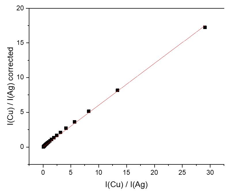
Plotting the corrected
ratios over the simulated ratios yields a straight line through
the origin (figure 10), indicating that all values can be
transformed using the same correction factor over the whole
concentration range. The correction factor
This result shows that
correction factors for XRF measurements can not only be
developed via the experimental route using reference samples as
written in section 3.1.1. but also by simulations.
3.3. Influence of
sample geometry (embossing) of coins on the accuracy of the
results
In the following section
the influence of different angles of incident beam will be
shown. To investigate this phenomenon the composition of the
simulated coin was kept the same, while the angle of the
incident beam was varied. The following table 6 shows the
different intensities of induced Cu and Ag X-rays as well as the
ratio between these intensities. The simulated setup of the
XRF-spectrometer stayed the same, meaning that the detector
stayed in the same position regarding the X-ray-tube. This leads
to the detector changing its angle to the simulated sample with
the X‑ray‑tube.
|
Angle of
incident X-ray beam |
I(Cu) |
I(Ag) |
I(Cu) / I(Ag) |
|
-60° |
52001 |
42424 |
1.23 |
|
-50° |
47334 |
39666 |
1.19 |
|
-45° |
45530 |
38542 |
1.18 |
|
-40° |
43940 |
37485 |
1.17 |
|
-30° |
41065 |
35657 |
1.15 |
|
-20° |
38603 |
34014 |
1.13 |
|
-10° |
36162 |
32372 |
1.12 |
|
0° |
33773 |
30657 |
1.10 |
|
10° |
31137 |
28747 |
1.08 |
|
20° |
28127 |
26448 |
1.06 |
|
30° |
24355 |
23443 |
1.04 |
|
40° |
19154 |
18910 |
1.01 |
|
45° |
15697 |
15586 |
11.01 |
The ratio of intensities
between Cu and Ag radiation changes with different angles of
incident X‑ray beam. This means that the elements Cu and Ag are
affected in different ways by the different measurement
geometries. Radiation with higher energy can pass more material
than radiation with lower energy. This might be the reason the
geometric effect is stronger for Cu than for Ag, because the Ag
fluorescence has higher energies. The geometric effect will
probably account for a large part of the uncertainties of single
XRF measurements. This effect can be seen in the plot in
figure 11.
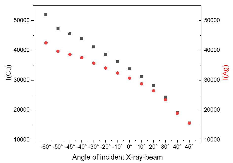
Figure 11
shows the plot of Cu and Ag intensities over the angle of
incident X-ray beam. The geometric effect is clearly visible
with both elements but seems to be stronger for Cu than it is
for Ag. With a very flat angle and the detector being almost
perpendicular to the sample, this leads to a stronger
overrepresentation of the element with lower energy radiation,
because less thickness of the sample needs to be passed and the
detector has an advantageous position. The general decline of
intensity from -60° to +45° might come from the positioning of
the detector to the sample. This result is of consequence in the
case of irregular surfaces, like coins, as sketched in figure
4. Obviously, as documented in table 6, the influence
of the exact surface geometry of a sample on the measured Cu/Ag
ratio can be as much as 20%. This is comparable to the factual
difference of measurements between two points of the same coin.
Thus, we conclude that
the difference of measurement results from different points of
the same coin is mainly caused by the surface geometry of the
coins. In consequence, if a coin is measured with a portable
XRF, it is good practice to measure several points and calculate
average concentrations (as it is done throughout this work) to
obtain more reliable (precise) results. The uncertainty of these
average values will reflect the geometric effect described
above.
3.4. Application of a
correction factor in the investigation of billon coins
The billon coins were
measured in the way mentioned in section 2.3. The obtained
concentrations were adjusted applying the correction factor for
Ag and Cu, respectively. Ten measurements per side of the coin
were undertaken, totaling at 20 measurements for each coin. The
results are given in table 7. On first sight, the
compositions are typical billon materials within a narrow range
of Cu/Ag ratios. Also, the data of the trace elements show no
obvious trend. However, we plotted these data for each possible
pair of elements. These plots were investigated via Pearsons’s
R, a statistical measure for the correlation of two components.
This method is often used for handling large sets of data. A
large set of data was collected to have more precise data. In
this case we made use of Pearsons’s R to identify possible links
between different elements of the coins.
|
Sample |
Cu/wt% |
Ag/wt% |
Au/wt% |
Fe/wt% |
Zn/wt% |
Sn/wt% |
Pb/wt% |
|
Claudius |
|||||||
|
ALSK_0047 |
2.88 |
95.38 |
0.41 |
0.06 |
0.03 |
0.62 |
0.63 |
|
ALSK_0048 |
29.14 |
69.31 |
0.28 |
0.06 |
0.19 |
0.53 |
0.49 |
|
ALSK_0058 |
46.51 |
51.62 |
0.32 |
0.11 |
0.49 |
0.6 |
0.35 |
|
ALSK_0059 |
59.8 |
38.22 |
0.36 |
0.1 |
0.66 |
0.64 |
0.21 |
|
ALSK_0060 |
36.42 |
61.96 |
0.27 |
0.15 |
0.28 |
0.52 |
0.4 |
|
AL_0061 |
63.66 |
34.07 |
0.26 |
0.13 |
0.88 |
0.42 |
0.58 |
|
AL_0062 |
47.03 |
51.28 |
0.28 |
0.1 |
0.48 |
0.62 |
0.2 |
|
AL_0063 |
30.52 |
67.35 |
0.38 |
0.1 |
0.28 |
0.73 |
0.64 |
|
AL_0064 |
68.59 |
29.35 |
0.18 |
0.15 |
0.86 |
0.49 |
0.39 |
|
AL_0065 |
42.74 |
54.59 |
0.42 |
0.18 |
1.32 |
0.41 |
0.33 |
|
AL_0075 |
64.9 |
33.25 |
0.23 |
0.15 |
0.77 |
0.39 |
0.32 |
|
AL_0076 |
68.33 |
29.77 |
0.22 |
0.12 |
0.78 |
0.34 |
0.45 |
|
AL_0081 |
30.07 |
68.28 |
0.4 |
0.08 |
0.55 |
0.41 |
0.21 |
|
AL_0082 |
67.46 |
30.66 |
0.36 |
0.1 |
0.84 |
0.37 |
0.21 |
|
AL_0086 |
58.39 |
39.69 |
0.13 |
0.12 |
0.85 |
0.52 |
0.31 |
|
AL_0087 |
53.01 |
41.99 |
0.45 |
0.41 |
3.55 |
0.32 |
0.27 |
|
AL_0088 |
36.72 |
60.56 |
0.27 |
0.08 |
0.8 |
0.58 |
0.99 |
|
Nero |
|||||||
|
AL_0187 |
77.2 |
21 |
0.13 |
0.28 |
0.86 |
0.31 |
0.23 |
|
AL_0188 |
73.62 |
24.54 |
0.24 |
0.18 |
0.74 |
0.36 |
0.32 |
|
AL_0189 |
56.06 |
41.81 |
0.29 |
0.17 |
0.51 |
0.67 |
0.48 |
|
ALSK_0169 |
77.54 |
20.61 |
0.13 |
0.12 |
0.96 |
0.43 |
0.21 |
|
ALSK_0170 |
76.7 |
20.74 |
0.1 |
0.94 |
0.76 |
0.44 |
0.32 |
|
ALSK_0171 |
46.06 |
52.08 |
0.48 |
0.09 |
0.47 |
0.66 |
0.16 |
A value of 1 means a
full positive correlation between two components, while a value
of -1 indicates a full negative correlation. It turned out that
most elements showed no correlation, except between Cu, Ag (the
main components) and the trace element Au (see table 7).
|
Pearson’s R |
All billon coins |
Nero |
Claudius |
|
Rxy/Cu(Ag) |
-0.999 |
-0.999 |
-0.998 |
|
Rxy/Cu(Au) |
-0.546 |
-0.817 |
-0.420 |
|
Rxy/Ag(Au) |
0.534 |
0.816 |
00.403 |
Pearson’s R suggests that there are several correlations within the sample set. In principle such correlations could be used to differentiate between sample groups that are different due to production method, provenience, used raw materials, etc. The two main components of these coins are Cu and Ag. A fully negative correlation is to be expected and is also shown in Pearson’s R with values of -0.999 and -0.998 respectively for both Claudius and the Nero coins. Interestingly, there is also a positive correlation between Ag and the trace element Au that can be seen from the data (and, consequently, a negative correlation between Cu and Au). Within the sample set of emperor Claudius, the correlation is smaller with a value of 0.403 than compared to the sample group of emperor Nero with 0.816 (see figure 12). The correlation between these two elements is evident in both sets of coins but is stronger (larger R value) for the coins of the Nero era. A correlation value of +1 would mean that every time a larger Ag value is measured, the Au value must also be larger. This is not the case for every measurement in our research, but this underlying trend was more often found in the Nero group as it was in the Claudius group, leading to the higher value for Pearson’s R. The difference in correlation values may be an indicator to different origins of the metal ore, a different production site, or maybe recycling of some valuables into coins. But this would have to be reassured by other indicators as well.
While we have no
immediate reason or interpretation at hand why these sample sets
are different both groups can be divided from each other using
this correlation as a criterion. This may be explained by the
sample group, which is 2.5 times larger for Claudius than for
Nero, which may result in a stronger correlation value.
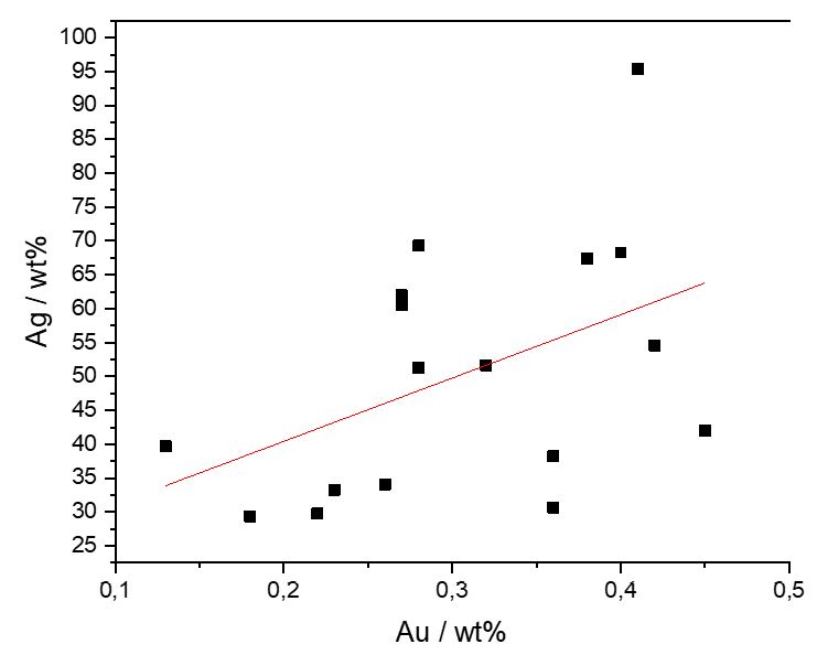
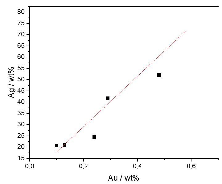
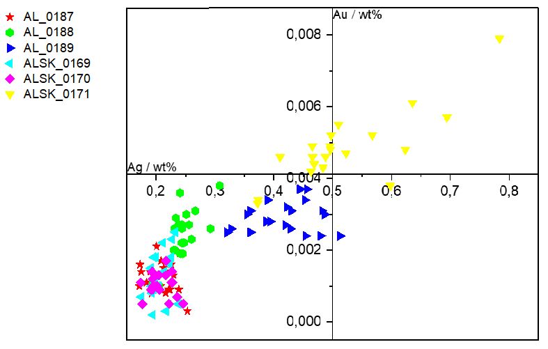
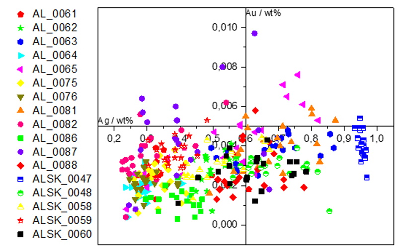
Further, if not only the
averaged Ag/Au concentrations of the coins are plotted but the
individual measurements (color-coded in figure 13), it
can be seen that the subset of Nero coins clearly shows a
division into two clusters (figure 13, right side), where
one group has lower silver and gold contents and the other group
has larger silver and gold concentrations. Although there is
some scattering of the single measurements, each coin falls
clearly in one of these 2 clusters. An explanation for these
different clusters must in any case lie in the different
material compositions; more extensive serial examinations using
this analytical method could perhaps develop further hypotheses
about the different origins of the raw materials or certain
manufacturing mechanisms in the minting of the coins.
4. Conclusion
This work shows that the
accuracy of data obtained through XRF-measurement can be
improved by applying correction factors. Such correction factors
can be obtained either by using reference samples as well as by
simulations. A correction factor
= 0.602
for copper in billon
coins was obtained from simulations with XMI-MSIM. With
reference samples, a correction factor regarding the wt% amount
of lead in lead-bronze coins was obtained. The value of this
correctional factor
is (1)
= 1.84
Simulations were also
used to estimate the influence of sample surface geometry. It
can be concluded that the variance of single measurements on the
same coin can be interpreted as measurement effects due to
irregular surfaces. This effect influences precision, but
precision can be increased by a larger data set.
All in all, while the
accuracy of portable XRF remains an issue, enough single
measurements on the same object will yield sufficient precision
to enable meaningful comparisons of coins, especially groups of
coins. This might offer new insights on a set of coins and might
open new perspectives if many samples (coins) are analyzed,
which is relatively easy with portable XRF.
A drawback for measuring
coins might be the fact that elemental composition of coins is
not homogenous regarding core and outer shell. The works of
Damian Gore and Gillan Davis[21]
suggest that especially for Ag containing coins the composition
between core and shell differs. On the outside the content is
usually significantly higher than in its core. Also, Gore and
Davis have suggested mathematical modelling for correcting the
data given by XRF. This is further strengthened by Gölitzer[22].
But these works also indicate a correlation between Ag content
of core and shell of a coin. This means if the outer shell of a
coin is measured more precisely, also the core data becomes more
precise as well. Of course, some accuracy is lost but for the
comparison of coins and coin groups, accuracy is of less
importance than precision. Gore compared XRF data with
destructive techniques (ICP-MS) to verify his findings, also
improving accuracy, but in our view, this is no prerequisite for
the analysis of composition trends. Because XRF using portable
spectrometers is possible within a museum environment and a
single measurement is very fast (a few minutes), many samples
and many measurements on one sample can be measurements, which
is a unique advantage to other methods. The larger the datasets,
the easier it is to identify groups or show (yet unknown) trends
within groups. Even if other methods, especially destructible
methods, yield more accurate results, this shows the
advantageous application of relatively simple X-ray equipment.
We would like to emphasize these strengths of portable XRF,
underpinning e.g. previous examples referred to by Liritzis and
Zacharias[23],
although other, partially more accurate and precise, analytical
methods are at hand.
All in all, this work
shows that especially when correction factors are applied, it is
possible to use XRF successfully for the elemental
characterization of coins. Correction factors are needed to
obtain more accurate results, especially for the main components
of the coins, while the analysis of trace amounts is not
influenced as strongly. A sufficient number of single
measurements with portable XRF improves precision sufficiently,
providing easy access to measurement of high sample numbers with
the potential to discover yet unknown trends in composition.
[1]
Zmuda-Trzebiatowska et al. 2019; Van Ham-Meert et al.
2020; Mozgai et al. 2021; Wallace et al. 2021,
343–371.
[2] Houk et
al. 1980, 2283–2289.
[3] Boumans
– Vrakking 1987a, 819–840; Boumans – Vrakking 1987b,
553–579; Boumans – Vrakking 1987c, 513–525.
[4] Kusko et al. 1990,
49. 288–292
[5] Jarvis – Williams
1993, 251–262.
[6] Kusko et al. 1990,
49. 288–292.
[7] Proctor
– Yu 1950, 717–717.
[8] Pimentel
1960, 651.
[9]
Hoyo-Meléndez 2017, 257–262.
[10]
Greenberg et al. 2011, 193–207.
[11] Gordus
et al. 1967, 87–96.
[12] Guerra
et al. 2008, 2334–2338; Reiche et al. 2004, 83–91;
Alfeld 2020, 72–75; Vittiglio et al. 1999, 1697–1710.
[13]
Shackley 2011, 1–6.
[14]
Johansson 1989, 48–53; Malmqvist et al. 1989, 685–689;
Johansson 1990, 167–188.
[15] Guerra
et al. 2008, 2334–2338; Reiche et al. 2004, 83–91.
[16] Vincze
et al. 1993, 553–573; Vincze et al. 1995a, 1481–1500;
Vincze et al. 1995b, 127–147; Vincze et al.
1999, 1711–1722; Schoonjans et al.
2012, 10–23; Schoonjans et al. 2013, 36–41.
[17] Moseley 1913,
1024–1034; Moseley 1914, 703–713.
[18] Broll 1986,
271–285.
[19] Gölitzer 2004,
25–59.
[20] Denker et al.
2005, 65–70.
[21]
Gore – Davis 2016, 840–851; Davis et al.
2020.
[22] Gölitzer 2004,
25–59.
[23] Liritzis –
Zacharias 2011, 109–142.